2.1. The Jansen-Rit Neural Mass Model

Here, we will introduce the Jansen-Rit model, a neural mass model of the dynamic interactions between 3 populations:

pyramidal cells (PCs)

excitatory interneurons (EINs)

inhibitory interneurons (IINs)

Originally, the model has been developed to describe the waxing-and-waning of EEG activity in the alpha frequency range (8-12 Hz) in the visual cortex [1]. In the past years, however, it has been used as a generic model to describe the macroscopic electrophysiological activity within a cortical column [2]. A graphic representation of such a model, placed inside a brain network, can be found in the figure below.

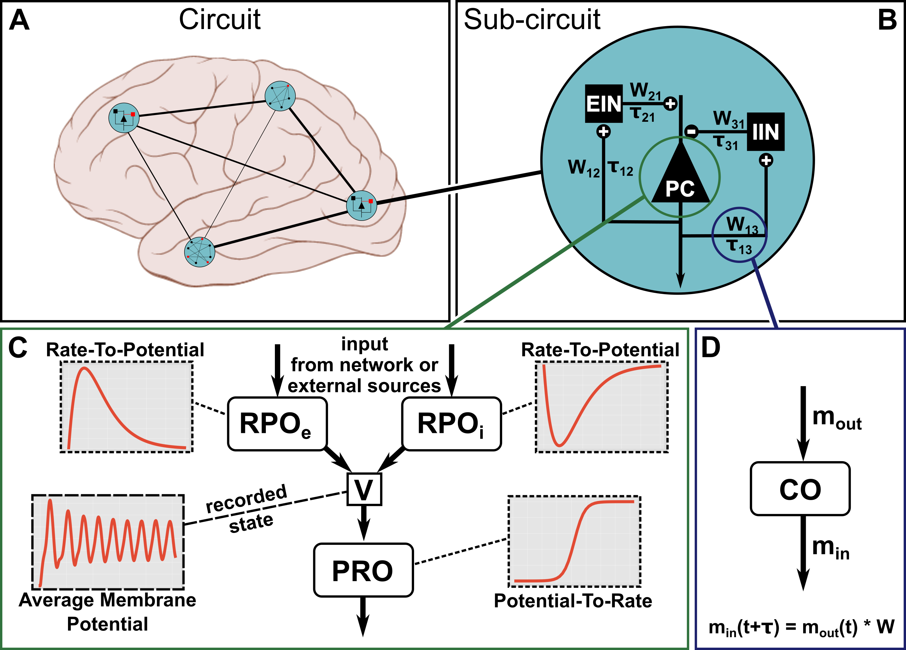
../_images/pyrates_model.png — Figure 1

The structure of the full Jansen-Rit model is depicted in Figure 1 B. As visualized for the pyramidal cell population in :ref:`fig1`C, the model can be decomposed into a number of generic mathematical operators that can be used to build the dynamic equations for the Jansen-Rit model. Essentially, the membrane potential deflections that are caused at the somata of a population by synaptic input, are modeled by a convolution operation with an alpha kernel. This choice has been shown to reflect the dynamic process of polarization propagation from the synapse via the dendritic tree to the soma [3]. The convolution operation can be expressed via a second-order differential equation:

\[ \begin{align}\begin{aligned}\dot V &= I,\\\dot I &= \frac{H}{\tau} m_{in} - \frac{2 I}{\tau} - \frac{V}{\tau^2},\end{aligned}\end{align} \]

where \(V\) represents the average post-synaptic potential and \(H\) and \(\tau\) are the efficacy and the timescale of the synapse, respectively. As a second operator, the translation of the average membrane potential deflection at the soma to the average firing of the population is given by a sigmoidal function:

\[m_{out} = S(V) = \frac{m_{max}}{1 + e^{(r (V_{thr} - V))}}.\]

In this equation, \(m_{out}\) and \(V\) represent the average firing rate and membrane potential, respectively, while \(m_{max}\), \(r\) and \(V_{thr}\) are constants defining the maximum firing rate, firing threshold variance and average firing threshold within the modeled population, respectively.

By using the linearity of the convolution operation, the dynamic interactions between PCs, EINs and IINs can be expressed via 6 coupled ordinary differential equations that are composed of the two operators defined above:

\[ \begin{align}\begin{aligned}\dot V_{pce} &= I_{pce},\\\dot I_{pce} &= \frac{H_e}{\tau_e} c_4 S(c_3 V_{in}) - \frac{2 I_{pce}}{\tau_e} - \frac{V_{pce}}{\tau_e^2},\\\dot V_{pci} &= I_{pci},\\\dot I_{pci} &= \frac{H_i}{\tau_i} c_2 S(c_1 V_{in}) - \frac{2 I_{pci}}{\tau_i} - \frac{V_{pci}}{\tau_i^2},\\\dot V_{in} &= I_{in},\\\dot I_{in} &= \frac{H_e}{\tau_e} S(V_{pce} - V_{pci}) - \frac{2 I_{in}}{\tau_e} - \frac{V_{in}}{\tau_e^2},\end{aligned}\end{align} \]

where \(V_{pce}\), \(V_{pci}\), \(V_{in}\) are used to represent the average membrane potential deflection caused by the excitatory synapses at the PC population, the inhibitory synapses at the PC population, and the excitatory synapses at both interneuron populations, respectively.

Below, we will demonstrate how to load this a model into pyrates and perform numerical simulations with it.

References

2.1.1. Step 1: Importing the frontend class for defining models

As a first step, we import the pyrates.frontend.CircuitTemplate class, which allows us to set up a model definition in PyRates.

from pyrates.frontend import CircuitTemplate

2.1.2. Step 2: Loading a model template from the model_templates library

In the second step, we load a model template for the Jansen-Rit model that comes with PyRates via the from_yaml() method of the CircuitTemplate. This method returns a CircuitTemplate instance. Have a look at the yaml definition of the model that can be found via the path used for the from_yaml() method. You will see that all variables and parameters are already defined there. As an alternative, you can also use the circuit_from_yaml() function that you can simply import via from pyrates import circuit_from_yaml. These are the basic steps you perform, if you want to load a model that is defined inside a yaml file. To check out the different model templates provided by PyRates, have a look at the PyRates.model_templates module.

jrc = CircuitTemplate.from_yaml("model_templates.neural_mass_models.jansenrit.JRC")

2.1.3. Step 3: Numerical simulation of a the model behavior in time

After loading the model template, numerical simulations can be performed via the run() method. Calling this function will solve the initial value problem of the above defined differential equations for a time interval from 0 to the given simulation time. This solution will be calculated numerically by a differential equation solver in the backend, starting with a defined step-size. As part of this process, a pyrates.backend.BaseBackend instance is created that contains a graph representation of the network equations. How exactly these equations will be solved, can be customized via the arguments of the run() method. You can choose between different backends, numerical solvers and integration step-sizes, for instance. Here, we choose the scipy backend, which uses a 4(5)th order Runge-Kutta method as default numerical solver. The default of the run() method is the forward Euler method that is implemented in PyRates itself.

results = jrc.run(simulation_time=2.0,
                  step_size=1e-4,
                  sampling_step_size=1e-3,
                  outputs={'V_pce': 'pc/rpo_e_in/v',
                           'V_pci': 'pc/rpo_i/v'},
                  backend='default',
                  solver='scipy')

2.1.4. Step 4: Visualization of the solution

The output of the run() method is a pandas.Dataframe, which comes with a plot() method for plotting the timeseries it contains. This timeseries represents the numerical solution of the initial value problem solved in step 4 with respect to the state variables \(V_{pce}\) and \(V_{pci}\) of the model.

import matplotlib.pyplot as plt
plt.plot(results)

To visualize the average membrane potential at the PC somata, simply plot the sum of the excitatory and inhibitory post-synaptic potentials \(V_{pce}\) and \(V_{pci}\):

v_pc = results['V_pce'] + results['V_pci']
plt.plot(v_pc)
plt.legend(['V_pce', 'V_pci', 'V_pce - V_pci'])
plt.ylabel('V')
plt.xlabel('time')

plt.show()

Gallery generated by Sphinx-Gallery